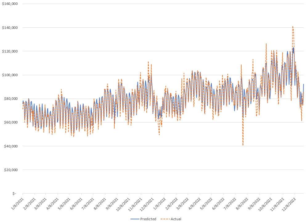
A sample of the production code for a deep neural net time series model. In general, it achieved over 95% accuracy in predicting ad revenue.

Background

Our clients needed to forecast revenue trends, so they could make necessary adjustments across media channels. To address this, I developed a deep neural net time series model.

Methodology

The deep neural net time series model used the Keras package, which is a wrapper for Tensorflow. Specifically, the model was a LSTM Recurrent Neural Networks¹. These models are powerful tools for modeling sequential data, especially when dealing with long-term dependencies, such as those found in time series data.

The process in building the model follows your usual machine learning process.

First, I ingested the data using a SQLAlchemy connection to our database.

Next, I cleaned the data:

Removed special characters from text fields.
Ensured correct input for categorical variables.

Then, as this was a time series, I feature engineered additional time-based variables. This included categorical variables for:

Holidays
Weekends

Afterward, I preprocessed the data:

Created embeddings for categorical data.
Restructured categorical data.
Restructured continuous data.

Now that the data was ready for modeling, I split the data into test and train.

When creating the time series model, I ran a grid search over several factors:

Number of nodes
Number of levels
Dropout rate
Validation samples

For clarity, here’s a sample of the modeling code.

input_all = concatenate([embeds[0], embeds[1], embeds[2],
  embeds[3], embeds[4], embeds[5],
  input_cnt])
visible_all = LSTM((int(lstm_nodes)), activation='relu', return_sequences=True)(input_all)
hidden1_all = LSTM((int(lstm_nodes / 2)), activation='relu', return_sequences=True)(visible_all)
hidden2_all = LSTM((int(lstm_nodes / 4)), activation='relu', return_sequences=True)(hidden1_all)
hidden3_all = LSTM((int(lstm_nodes / 8)), activation='relu', return_sequences=True)(hidden2_all)
hidden4_all = LSTM((int(lstm_nodes / 16)), activation='relu', return_sequences=True)(hidden3_all)
hidden5_all = LSTM((int(lstm_nodes / 8)), activation='relu', return_sequences=True)(hidden4_all)
hidden6_all = LSTM((int(lstm_nodes / 4)), activation='relu')(hidden5_all)
dropout_all = Dropout(n_drop)(hidden6_all)
model_all = Model(inputs=[inputs[0], inputs[1], inputs[2],
  inputs[3], inputs[4], inputs[5],
  input_cnt],
  outputs=[output_all])
model_all.fit([df_cat[0], df_cat[1], df_cat[2],
  df_cat[3], df_cat[4], df_cat[5],
  df_cnt],
  df_y, epochs=(int(n_epochs)),
  batch_size=(int(n_batch)),
  callbacks=[
  EarlyStopping(monitor='loss', patience=10)],
  verbose=0,
  shuffle=False)

Once the best model was found, I created forecasts using the best parameters from the grid search.

For the finished product, I also created a simple function for the confidence bands:

To illustrate that as the forecasts move out in time, we become less confident in those forecasts, I created confidence bands around the forecast.

See below.

y_forecast = model.predict([df_cat_est_X_lst[0], df_cat_est_X_lst[1], df_cat_est_X_lst[2],
df_cat_est_X_lst[3], df_cat_est_X_lst[4], df_cat_est_X_lst[5],
df_cnt_est_X])
y_forecast_rescale = y_scaler.inverse_transform(y_forecast)
y_forecast_rescale = pd.DataFrame(y_forecast_rescale)
y_forecast_rescale.columns = ['Forcasted_Revenue']
for i in range(0, len(y_forecast_rescale)):
  if i < 90:
      y_forecast_rescale.loc[(i, 'Forecasted Min')] = int(y_forecast_rescale.loc[(i, 'Revenue')] - 1 * rev_std - 2 * (i / 90) * rev_std)
      y_forecast_rescale.loc[(i, 'Forecasted Max')] = int(y_forecast_rescale.loc[(i, 'Revenue')] + 1 * rev_std + 2 * (i / 90) * rev_std)
  if i >= 90:
      y_forecast_rescale.loc[(i, 'Forecasted Min')] = int(y_forecast_rescale.loc[(i, 'Revenue')] - 1 * rev_std - 2 * rev_std)
      y_forecast_rescale.loc[(i, 'Forecasted Max')] = int(y_forecast_rescale.loc[(i, 'Revenue')] + 1 * rev_std + 2 * rev_std)

Results and Analysis

To assess the model’s accuracy, I compared its predictions to the actual value.

As you can see, the time series model using LSTM Recurrent Neural Networks did well. image-center

As an added value, I provided the relative importance of the input variables to guide our clients’ decision-making. This was accomplished using Shapley values.

Conclusion

This project successfully developed a deep neural network time series model using LSTMs to forecast revenue trends for our clients. By leveraging Keras and a well-defined machine learning workflow, the model effectively captured the sequential nature of the data and learned from long-term dependencies. The implemented grid search ensured optimal hyperparameter selection, leading to accurate forecasts with confidence bands. Additionally, analyzing relative feature importance via Shapley values provided valuable insights for client decision-making across media channels.

Previous Next

The model was built from scratch and leveraged the work by Jason Brownlee. ↩

A Deep Neural Net Time Series Model

Jonathan Manalo

Background

Methodology

Results and Analysis

Conclusion